Introduction to Image Transforms

Image processing is a fun topic that sets the stage for learning machine vision. Whenever learning the MATLAB image processing tool bench, one way to experiment with manipulation is to morph yourself into a pug.

Why? Well, along with being delightful creatures, it allows for a way to explore geometric constraints between different photographs. The result will be an animation showing you the transformations required to match these geometric constraints to each other.

First, let's consider any generic image. It's a collection of points that can be represented as a matrix. For our purposes, we can consider it to be:

X  holds the x-coordinates of all pixels. Y holds the y-coordinates of all pixels. Each color channel is numbered (1 for grayscale or 3 for RGB or whatever scheme you're using. The value of any given point corresponds to the darkness on that color channel. 255 on a gray channel means it's white, whereas 0 means it's black. On an RGB wheel, 255 indicates maximum darkness for that channel. For example, maximum red and green make yellow. For those playing with hexadecimal notation, this would be #FFFF00, where F means the hex digit 16.

Make sense so far? Awesome.

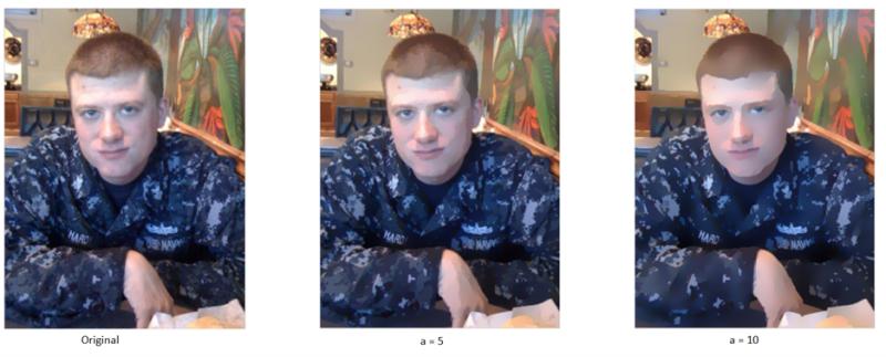
Okay, let's say we want to double the overall size of the image. We could multiply every point by an identity matrix with a scalar 2 applied. That was a bit to take in, but this is what it'd look like.

In case you're wondering, we're not messing with the color channel portion of the matrix, which is why it gets a 1 applied.

That covers increasing the size, but what if we want to stretch the image in one direction only? Easy, we drop the corresponding 2 and turn it into a 1.

Similarly, we could swap a value for 0.5 to compress in that direction.

Let's say we want to rotate the image next. We can multiply by our trigonometric matrix to rotate the image by an angle theta.

Naturally, you can skew the image by multiplying a scalar value by your trigonometric functions.

This covers our traditional image transformations but what about geometric constraints and the pug morph?

This actually goes into image stitching. If you've ever dealt with photogrammetry (using photographs in 3d imaging), you'll be used to attaching images together. In 3d, this is a bit complicated and we use coded targets to do this. However, in 2d space we can just easily pick some points with our mouse cursor.

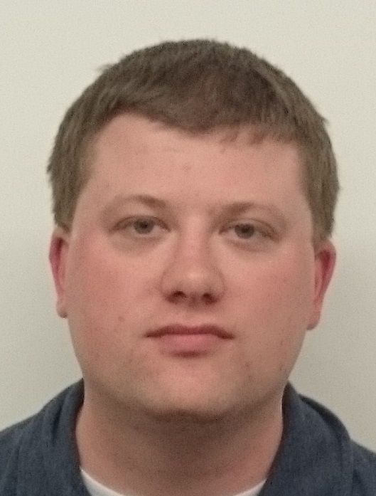
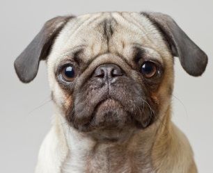
I'm going to show an image transform between my picture, above, to a pug shown at the top of the article.

MATLAB image processing toolbench allows you to directly do this with the Control Point Selection Tool.  We're going to transform based off of common points. For our purposes, we will be tying eyes together. Name the left eye P_LEFT and the right eye P_RIGHT.

Read your images in with this snippet:

A = imread('mypic.jpg');
B = imread('pug.jpg');
[m,n,k] = size(B);
A = imresize(A,[m,n]);
cpselect(A,B);

Whenever prompted, tie the left eye to the left pug eye, right eye to right pug eye, etc.

Export these points to your workspace.

At this point (pun, get it?), we're going to compute an affine transform to get from one image to the other. We will create a virtual control point using a little math. MATLAB's cp2tform will perform the control point alignment. However, your coordinate systems will not be matched up. We can realign the coordinate systems to a common frame with the align() procedure and throw that into a matrix.

Now we're going to write a little code:

for t=0:0.01:1
P_mid = (1-t)PA + tPB;
T_mid = cp2tform(PA, P_mid, 'affine');
[A2,B2] = align(A,B, T_mid);
I = (1-t)A2 + tB2;
imagesc(I); axis off; drawnow;
end;

Run this as a script. This will do a stepped transform using a cross-dissolve with each frame being created as it's displayed. If everything goes to plan, it should animate in a plot screen.