Gaussian Noise Detection and Removal in Imaging

The First Variation of Energy equation can be used for image denoising. I recently wrote an article that used a variation of that equation to focus on removing "salt and pepper" style image noise. This article looks at how to defeat "Gaussian" distribution noise in a color image.

Fundamentally, we will do something very similar to what we did for anisotropic filtering and salt and pepper denoising. Gaussian noise differs from salt and pepper noise in that it changes pixel values from 0-255 rather than setting them to either 0 or 255. As a result, our other filter will not work.

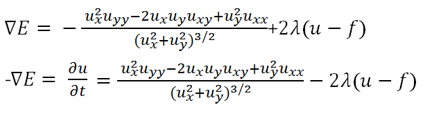
In this case, we will take the First Variation of Energy equation and change it around a little bit to find the minimum energy instead of the maximum energy of a system.

What does that do?

Well, consider a contour map of a mountain with a bunch of sharp spikes everywhere. That has a lot of energy. If we smoothed it and eliminated the sharp spikes, it would have less energy.

By taking the Heat equation for a 2d plane, applying Neumann boundary conditions, solving the partial differential equation, then taking the inverse of the result, we'll have an equation that gives us a stepped reduction in energy. If we take the original image, weight it by a fidelity factor, then shove that all into MATLAB, we get a chunk of the below code at the bottom of this article.

We'll then run the image, pixel-by-pixel, through our MATLAB function while taking the minimum energy each time. Again, recall that the original image is weighted by our lambda constant to ensure that we maintain image fidelity.

Each iteration of the TV Energy equation will smooth out the image. This will provide despeckling but also reduce image detail around sharp corners. We're basically trying to round off every sharp corner in the image, which removes individual noise speckles.

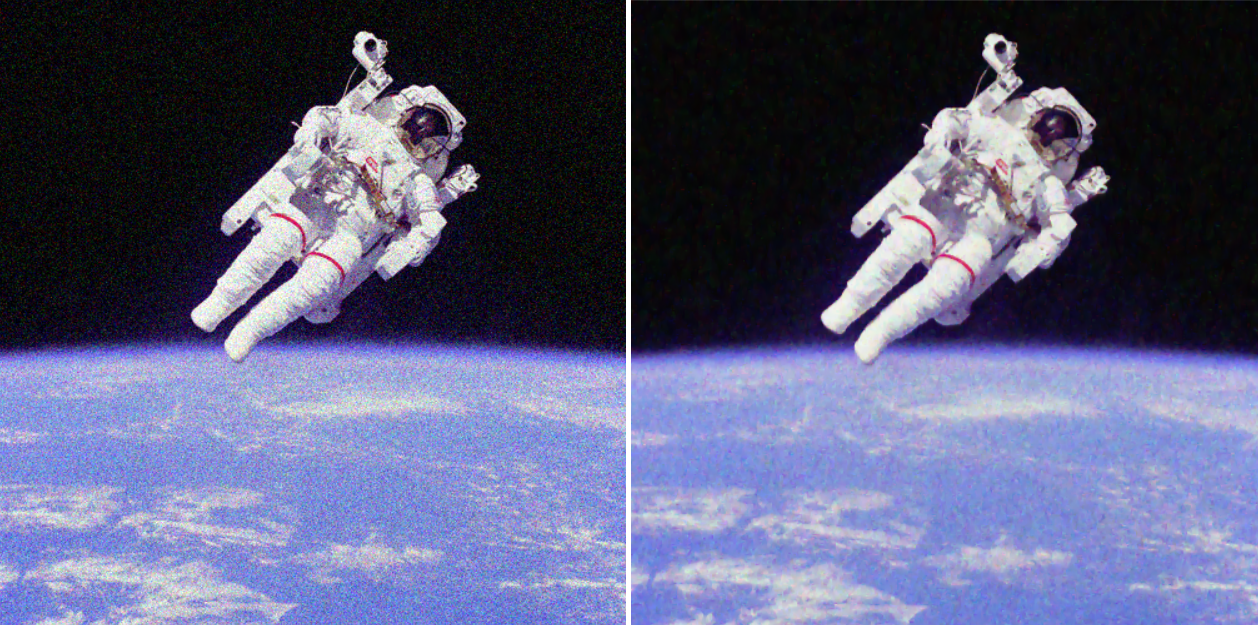
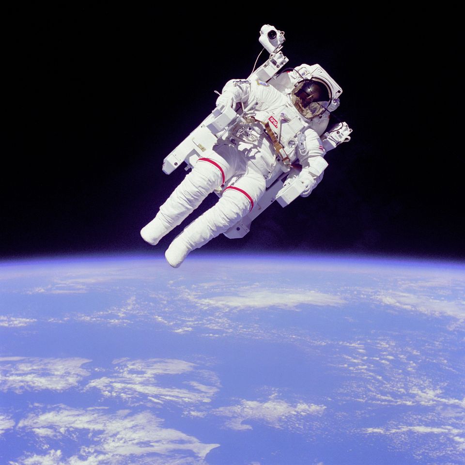
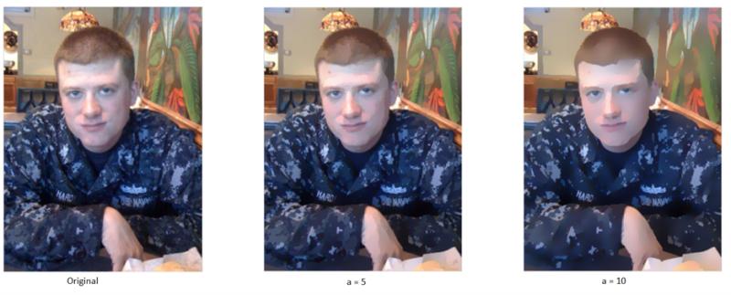
I took the featured image from the top of this article, applied Gaussian noise across all 3 color channels, then put it on the above-left image. I then ran that image through the TVEnergy function shown below. Inputting random values for lambda, I got the above-right image after some experimentation. With a lambda of around 0.01, I got a pretty high Signal to Noise ratio for this image compared to the original. Each image, naturally, will have its own best lambda value to get a clean result.

You'll note that this is not a perfect process, and some image fidelity is lost. That's an unfortunate result of the smoothing operation.

A = imread('yourimagehere.jpg'); % Load the image with this command at the command line
for i=1:3; C(:,:,i) = TVEnergy(A(:,:,i),0.01); end; % Call the function with this line, substituting your own lambda value as appropriate
function [u] = TVEnergy(f, lambda)
% Calculate TV energy value of an image.
% Author: Tyler Hardy
% www.wirebiters.com
% Input: Color image f
% Output: TV Energy of image f
set(gcf,'color','white'); % white background
f = double(f);
dt = 0.1;
T = 20;
u = f; % u will be modified. f will not be modified and will be used for image fidelity
for t = 0:dt:T % for loop **************
[m,n] = size(f);
% First center discrete derivatives
f_x = ( u(:,[2:n,n]) - u(:,[1,1:n-1]) ) / 2;
f_y = ( u([2:m,m],:) - u([1:m-1,1],:) ) / 2;
% Second derivative in x: f_xx
f_xx = u(:,[2:n,n]) - 2u + u(:,[1,1:n-1]);
% Second derivative in y: f_yy
f_yy = u([2:m,m],:) - 2u + u([1,1:m-1],:);
% Diagonal derivative f_xy
f_xy = (u([2:m,m],[2:n,n]) + u([1,1:m-1],[1,1:n-1])- u([1,1:m-1],[2:n,n])- u([2:m,m],[1,1:n-1])) / 4;
%Â Total Variation equation
u = u + dt.*((f_xx.f_y.^2 - 2f_x.*f_y.f_xy + f_yy.f_x.^2)./((f_x.2 +f_y.^2).(3/2)+0.1) - 2lambda.(u-f));
% Display the image
imshow(uint8(u)); title(t);
drawnow;
end % end for *************************
end % end function

If you want to use this code, please credit it per Creative Commons to this website. Images are Public Domain from NASA.